Python Backtesting with Claude (Anthropic): 5 Silent Overfitting Traps and the Deflated Sharpe Ratio
Quantitative audit of the 5 critical biases common in LLM-generated Python backtests (look-ahead bias, survivorship bias, data snooping, omitted slippage, train/test leakage), clean Python fixes, and Deflated Sharpe Ratio (DSR) math.
Last methodological review:

Quantitative Research · Quant Lab
Backtest & DSR Analyzer
Editorial illustration — TrueVerdikt
IN THIS ARTICLE
Key Takeaways (TL;DR)
- AI coding assistants like Claude dramatically speed up pandas/NumPy strategy prototyping, but routinely produce backtests with artificially inflated Sharpe ratios caused by silent implementation biases.
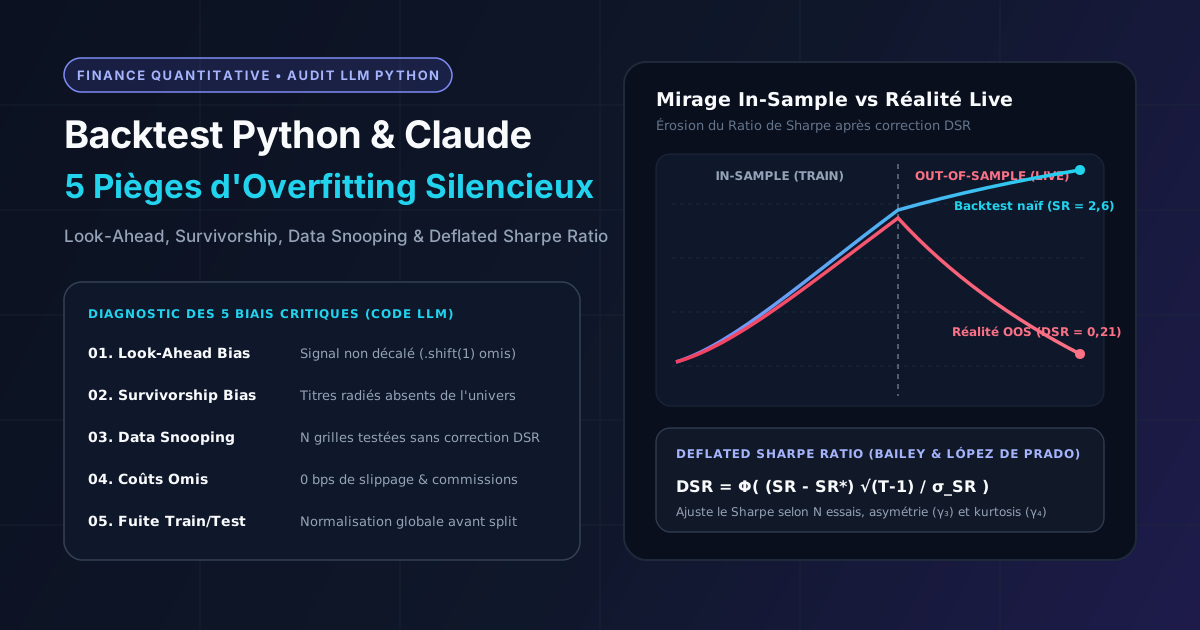
- Five traps account for most LLM backtest failures: look-ahead bias, survivorship bias, grid-search data snooping, omitted transaction costs, and train/test scaling leakage.
- The Deflated Sharpe Ratio (DSR) by Bailey and López de Prado adjusts observed performance for trial count N, return skewness, and excess kurtosis.
- Every Python strategy requires strict causal shifting (.shift(1)), realistic turnover-based slippage modeling, and purged walk-forward out-of-sample validation.
Advanced AI coding assistants such as Claude (Anthropic) have reshaped how quantitative researchers and systematic investors prototype trading ideas. Within seconds, a developer can generate clean pandas, numpy, and scipy scripts to test momentum, mean-reversion, or cross-sectional factor strategies.
Yet this acceleration exposes a classic paradox in financial econometrics: syntactically flawless Python code that executes without a single warning can still generate a mathematically invalid backtest. Because large language models (LLMs) optimize for readable, idiomatic software rather than market microstructure rigor, they frequently omit essential quantitative safeguards. The outcome is a textbook in-sample equity curve boasting a Sharpe ratio above 2.5 that collapses immediately in live out-of-sample trading.
This study dissects the 5 most frequent overfitting and data-leakage traps in LLM-assisted Python backtests, provides clean, production-grade Python corrections, and derives the Deflated Sharpe Ratio (DSR) to separate genuine statistical edge from random noise. You can audit your own return streams in our Backtest Analyzer and review statistical risk diagnostics inside the Quant Educator.
1. Trap #1: Look-Ahead Bias
Look-ahead bias occurs whenever a trading decision at time relies on information that is only observable at the close of bar (or later). In rapidly generated pandas backtests, the most prevalent bug is multiplying a signal computed from day 's closing price directly by day 's return, omitting .shift(1).
import numpy as np
import pandas as pd

def backtest_moving_average(close: pd.Series, fast: int = 20, slow: int = 100) -> pd.DataFrame:
    """Compare a look-ahead biased backtest against a strictly causal execution."""
    returns = close.pct_change().fillna(0.0)
    sma_fast = close.rolling(window=fast, min_periods=fast).mean()
    sma_slow = close.rolling(window=slow, min_periods=slow).mean()

    # Signal observed at the close of day t (1 = long, 0 = flat)
    raw_signal = (sma_fast > sma_slow).astype(float)

    # CLASSIC BUG: applies day t close signal to day t return
    biased_returns = raw_signal * returns

    # CAUSAL FIX: signal from close t is executed starting on day t+1
    causal_position = raw_signal.shift(1).fillna(0.0)
    valid_returns = causal_position * returns

    return pd.DataFrame(
        {
            "biased_equity": (1.0 + biased_returns).cumprod(),
            "valid_equity": (1.0 + valid_returns).cumprod(),
            "position": causal_position,
        }
    )
In short-horizon mean-reversion models (such as RSI or Bollinger Band triggers computed on daily closes), missing a single .shift(1) is enough to turn a losing strategy into a fictional +30% annualized return backtest.
2. Trap #2: Survivorship Bias
When prompted to backtest a multi-stock equity strategy on the S&P 500 or Nasdaq-100, an LLM will almost always scrape or hardcode the current list of index constituents (which includes today's mega-cap winners such as NVIDIA, Palantir, or CrowdStrike) and pull 10 to 15 years of historical prices.
This silently excludes every company that belonged to the index in 2012 or 2018 before going bankrupt, getting acquired at a distressed valuation, or being removed after an 80% drawdown. Retrospective survivor filtering routinely inflates historical annualized returns by 150 to 400 basis points—particularly in value and small-cap strategies—while severely understating historical Maximum Drawdown. Valid multi-asset backtests require a point-in-time constituent database that retains delisted securities and corporate actions.
3. Trap #3: Data Snooping and Multiple-Testing Bias
With Python and an AI assistant, running a nested grid search across or combinations of moving-average windows, volatility thresholds, and regime filters takes less than a minute. Selecting the single parameter pair that maximized the historical Sharpe ratio introduces severe selection bias.
Even if every tested rule is pure random noise with zero true alpha, the maximum Sharpe ratio observed across independent trials grows steadily with . To adjust for this inflation, David H. Bailey and Marcos López de Prado (2014) developed the Deflated Sharpe Ratio (DSR), which computes the probability that a strategy's true Sharpe ratio is strictly positive after accounting for the number of trials , sample length , skewness , and kurtosis .
First, we compute the expected maximum Sharpe ratio under the null hypothesis (zero true skill) across independent trials with cross-sectional variance :
where is the Euler-Mascheroni constant, is Euler's number, and is the inverse standard normal cumulative distribution function.
Next, the Deflated Sharpe Ratio evaluates the cumulative probability that the observed Sharpe ratio exceeds this noise threshold :
A strategy reporting a raw Sharpe ratio of 1.80 over trading days after searching configurations—especially with negative skewness () and fat tails ()—frequently drops to a DSR below 0.50, indicating statistical indistinguishability from luck.
import numpy as np
from scipy.stats import kurtosis, norm, skew

def deflated_sharpe_ratio(
    returns: np.ndarray,
    n_trials: int,
    sr_trials_std: float = 0.5,
) -> dict[str, float]:
    """Compute the Deflated Sharpe Ratio (Bailey & López de Prado, 2014)."""
    r = np.asarray(returns, dtype=float)
    r = r[~np.isnan(r)]
    t_obs = len(r)
    if t_obs < 30 or n_trials < 1:
        raise ValueError("Requires at least 30 observations and n_trials >= 1.")

    sr_obs = float(np.mean(r) / np.std(r, ddof=1))
    g3 = float(skew(r))
    g4 = float(kurtosis(r, fisher=False))  # Total kurtosis (3.0 for Gaussian)

    euler_gamma = 0.5772156649
    if n_trials == 1:
        sr_zero = 0.0
    else:
        z1 = norm.ppf(1.0 - 1.0 / n_trials)
        z2 = norm.ppf(1.0 - 1.0 / (n_trials * np.e))
        sr_zero = sr_trials_std * ((1.0 - euler_gamma) * z1 + euler_gamma * z2)

    denom = np.sqrt(max(1e-12, 1.0 - g3 * sr_obs + ((g4 - 1.0) / 4.0) * (sr_obs ** 2)))
    z_score = (sr_obs - sr_zero) * np.sqrt(t_obs - 1) / denom
    dsr_prob = float(norm.cdf(z_score))

    return {
        "sr_non_annualized": sr_obs,
        "sr_annualized": sr_obs * np.sqrt(252.0),
        "sr_threshold_zero": float(sr_zero),
        "dsr_probability": dsr_prob,
    }
4. Trap #4: Omitted Slippage, Commissions, and Turnover Drag
Most boilerplate backtests produced by LLMs evaluate gross returns without deducting execution costs. Whenever a strategy trades frequently, market microstructure frictions—bid-ask spreads, price impact (slippage), and brokerage commissions—compound rapidly against expected return.
Letting denote the target portfolio weight on day and the one-way proportional cost rate (for instance, , or 10 basis points per trade on liquid equities), net daily return must subtract absolute turnover :
import pandas as pd

def apply_transaction_costs(
    position: pd.Series,
    asset_returns: pd.Series,
    cost_bps: float = 10.0,
) -> pd.Series:
    """Deduct proportional commissions and slippage based on realized turnover."""
    cost_rate = cost_bps / 10_000.0
    turnover = position.diff().abs().fillna(position.abs())
    gross_returns = position.shift(1).fillna(0.0) * asset_returns
    net_returns = gross_returns - turnover * cost_rate
    return net_returns
A strategy executing 120 round-trip trades per year at a realistic 10 bps per side faces a deterministic annual drag of 2.40%—often enough to erase the entire theoretical alpha of a short-term mean-reversion rule.
5. Trap #5: Train/Test Temporal Leakage in Feature Scaling
When a Python backtest incorporates machine learning pipelines (scikit-learn, XGBoost, or regularized regressions), a subtle yet fatal error is applying feature standardization (StandardScaler().fit_transform(X)) or feature selection across the full dataset before splitting into training and testing windows.
Global scaling leaks future mean and variance statistics into historical rows. Similarly, applying shuffled cross-validation (KFold(shuffle=True)) to financial time series violates chronological causality, allowing the model to interpolate using observations occurring days after the target timestamp. Sound quantitative validation requires Purged Walk-Forward Validation with an embargo buffer, where every scaler, imputer, and hyperparameter is fit strictly on past training data (fit on train, transform on test).
6. Summary Matrix of the 5 Traps and Quantitative Fixes
| LLM Backtest Trap | Typical Python Code Symptom | Impact on Sharpe Ratio | Rigorous Quantitative Fix |
|---|---|---|---|
| 1. Look-Ahead Bias | signal * returns without shifting |
Extreme inflation (+1.0 to +3.0 SR) | Enforce .shift(1) on all close-derived signals and audit timestamps |
| 2. Survivorship Bias | Current S&P 500 / Nasdaq-100 list over 10+ yrs | Return overstatement (+1.5% to +4%/yr) | Use point-in-time historical constituents including delisted stocks |
| 3. Data Snooping | Grid search across parameter sets | Guaranteed false positives (in-sample) | Compute the Deflated Sharpe Ratio (DSR) and constrain parameter space |
| 4. Omitted Costs | Zero deduction on position.diff().abs() |
Mirage on high-turnover strategies | Model spread + slippage + commissions (5–25 bps one-way by liquidity) |
| 5. Train/Test Leakage | Global StandardScaler().fit_transform(X) or shuffle=True |
Artificial out-of-sample accuracy | Use purged Walk-Forward pipelines (fit strictly on past + embargo) |
7. Pre-Deployment Verification Checklist
Before trusting any Python backtest drafted with Claude or another LLM, apply this four-point verification protocol:
- Causality audit: Inspect every rolling indicator, signal shift, and rebalancing rule to verify that no bar- closing information is traded before .
- Cost stress test: Double
cost_bps(e.g., from 10 bps to 20 bps) and confirm whether the net Sharpe ratio remains economically meaningful. - DSR calculation: Log every trial explored during research honestly and evaluate your return series using our Backtest Analyzer.
- Strict out-of-sample holdout: Reserve an untouched recent window for final evaluation and use the Quant Educator to interpret skewness, tail risk, and drawdown duration.
LLMs are remarkable software engineering accelerators, but econometric discipline remains entirely the researcher's responsibility. That rigor is especially critical during volatility regime shifts—as underscored on November 19–20, 2026 by Anthropic's own volatile Nasdaq debut (ANT, +17% followed by -9% to -11%) and NVIDIA's ~14% weekly sell-off (NVDA): a strategy overfit to a calm bull regime routinely breaks the moment realized volatility and tail correlations spike.

Primary Academic Sources
- Bailey, D. H., & López de Prado, M. (2014) — "The Deflated Sharpe Ratio: Correcting for Selection Bias, Backtest Overfitting, and Non-Normality", The Journal of Portfolio Management, 40(5), 94–107.
- Harvey, C. R., Liu, Y., & Zhu, H. (2016) — "... and the Cross-Section of Expected Returns", The Review of Financial Studies, 29(1), 5–68.
- López de Prado, M. (2018) — Advances in Financial Machine Learning, John Wiley & Sons (chapters on Purged K-Fold Cross-Validation and Backtest Overfitting).
- Bailey, D. H., Borwein, J., López de Prado, M., & Zhu, Q. J. (2017) — "The Probability of Backtest Overfitting", Journal of Computational Finance, 20(4), 39–69.
Analytical Disclaimer: The Python implementations and econometric formulas in this article are provided solely for educational and methodological purposes. Simulated backtest performance does not guarantee future results and does not constitute personalized investment advice.
Backtest & DSR Analyzer
Audit Deflated Sharpe Ratio, Monte Carlo distributions, and selection bias directly on your return series.
Analyze a BacktestIndependent financial engineer based in Quebec, Canada, Alain Legrand builds and audits TrueVerdikt's deterministic models: Series A/F mutual fund vs. TSX ETF fee comparisons, RRSP/FHSA tax arbitrage, Canadian mortgage actuarial schedules, and statistical overfitting detection (Deflated Sharpe Ratio & CPCV).
Primary Regulatory & Academic Sources
- OSFI — Guideline B-20 (Residential Mortgage Underwriting) — Residential mortgage underwriting practices, procedures, and minimum qualifying rate stress-test.
- CRA — FHSA, RRSP & Home Buyers' Plan — Official contribution limits ($8,000/yr, $40,000 lifetime FHSA cap), tax deductions, and HBP repayment rules.
- CIFSC — Canadian Investment Funds Standards Committee — Standardized classification of Canadian mutual funds and ETFs used across our MER fee comparator.
- Bailey & López de Prado (2014) — The Deflated Sharpe Ratio — Correcting for Selection Bias, Backtest Overfitting, and Non-Normality. The Journal of Portfolio Management, 40(5), 94–107 (SSRN).
Keep reading
All articles in this section « Quant trading » →
Leveraged NVIDIA ETFs (NVDL, NVDX): Volatility Decay Math and Python Simulation of the -14% Sell-Off
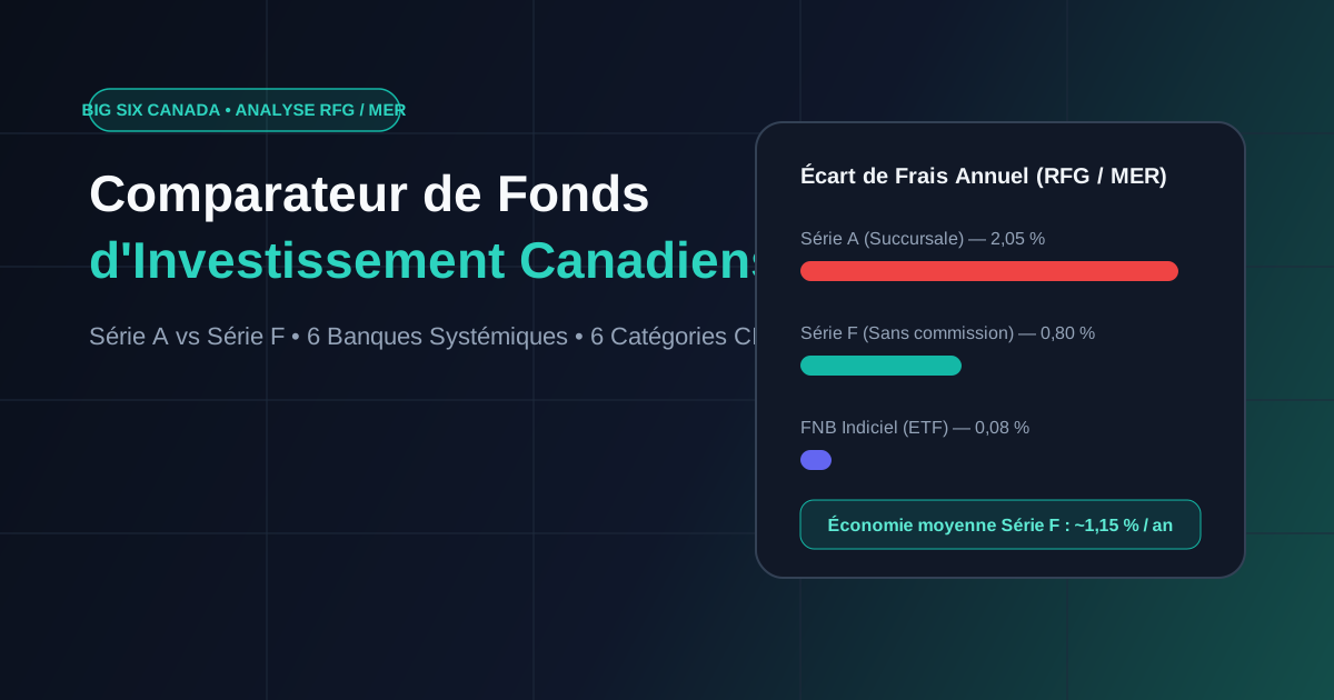
Canadian Investment Funds: How Big Six Bank Management Fees (MER) Silently Drain Your Portfolio (and How to Compare Them)